Modeling the plant (DC motors + wheels)
The goal of this second part is to obtain a model of 2 motors with wheels. So, we are going to work with math, don’t worry, it’s not to much.
First step is to run a program on the beaglebone in order to get the step response of a DC motor with a wheel, for this we need everything connected to the board (motor + encoder). Then we use a python script to fit the samples, which are the output of the previously run program, and with help of the same script we get the space state representation of the model. Finally we expand the representation for 2 motors.
Again here is the link to the git repo.
Step response of the plant
The space state representation of a DC motor model can be found here. Our plant also has a reduction gearbox, so the model takes the following form:
$$ A = \begin{pmatrix} 0 & 1 \\ a & b \end{pmatrix} $$ $$ B = \begin{pmatrix} 0 \\ c \end{pmatrix} $$ $$ C = \begin{pmatrix} 1 & 0 \end{pmatrix} $$
With help of scripts/stepResponse.py, we’ll find the values of a, b and c.
Getting the step response
As mention in the beginning, this is divided into 2 parts: run a program on the beaglebone and then analyzing its output with an script.
The program that runs on the board is called motor-step-response. Following the building instructions of the readme, we compile it as:
cd build
make -j motor-step-response
In a similar manner as motion-control, we should copy the binary with scp and
execute it being logged with ssh. In order to save the output on a file, we run:
./motor-step-respose > samples
Then we have to move samples from the beaglebone to our computer and run the script:
./scripts/stepResponse.py path/to/samples
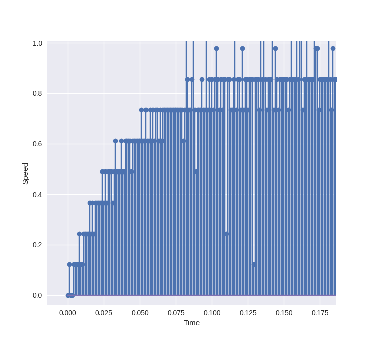
You will see all samples on a graph. Next step is fitting a curve.
Curve fitting
To accomplish the fitting of the step response 2nd order system with no overshoot, we need to get: the steady-state gain, time to 25% and time to 75% from the graph.
But it would be better if a moving average filter is applied on the samples:
./scripts/stepResponse.py -s 10 path/to/samples
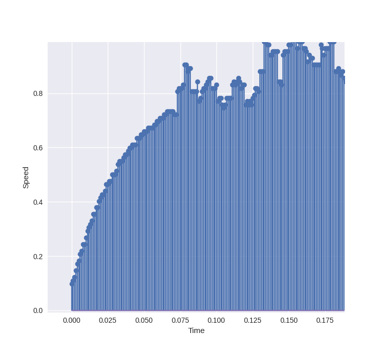
Now it’s easier to find the needed values:
| Parameter | Value |
|---|---|
| steady-state gain | 0.91 |
| time to 25% | 6.9 ms |
| time to 75% | 51.36 ms |
We can run the script again but this time with the parameters as arguments and we’ll obtain the transfer function and the state space representation:
./scripts/stepResponse.py -s 10 -c 0.91 6.9 51.36 path/to/samples
Battery Voltage: 8.18264[V]

            0.9100
------------------------------
   0.0002s^2 + 0.0364s + 1

A = [[0, 1], [-6279.911649874961, -228.7033441194173]]
B = [[0], [5714.719601386215]]
C = [1, 0]
From the output we have the values of a, b and c.
The complete model
This is the last part of this post and we are going to get the plant model for the 2 motors + wheels.
As first approach we can make one state space system with 2 inputs and 2
outputs from the original matrices A, B and C. The new matrices are:
$$ A = \begin{pmatrix} 0 & 1 & 0 & 0 \\ a & b & 0 & 0 \\ 0 & 0 & 0 & 1 \\ 0 & 0 & a & b \end{pmatrix} $$
$$ B = \begin{pmatrix} 0 & 0 \\ c & 0 \\ 0 & 0 \\ 0 & c \end{pmatrix} $$
$$ C = \begin{pmatrix} 1 & 0 & 0 & 0 \\ 0 & 0 & 1 & 0 \end{pmatrix} $$
Where the values of a, b and c are the same as before.
Further steps
Besides that you are able to verify the controllability and observability of the system with the above matrices, it is needed to rearrange them in order to implement a feedback loop. After doing some matrix transformations:
$$ A = \begin{pmatrix} 0 & 0 & 1 & 0 \\ 0 & 0 & 0 & 1 \\ a & 0 & b & 0 \\ 0 & a & 0 & b \end{pmatrix} $$
$$ B = \begin{pmatrix} 0 & 0 \\ 0 & 0 \\ c & 0 \\ 0 & c \end{pmatrix} $$
$$ C = \begin{pmatrix} 1 & 0 & 0 & 0 \\ 0 & 1 & 0 & 0 \end{pmatrix} $$
The method used for the control loop is pole placement. This requires to measure all the state variables but in case of 3WheelsBot the only measured variables are the angular velocity of the wheels. For this reason a reduced order observer was calculated (you can find this last on this jupyter notebook).
The library miLoCo has several control algorithms, also known as tasks. In case of pole placement with reduced observer, the indicated task is this.
After all calculation was done I decided to do a software in the loop test, i.e. to test the control loop with a simulated plant. I did this only for one motor here. You can compile this program and then run it on your computer (it is not needed to cross compile it).
In the next post, I will describe the software implementation required to get running the miLoCo’s task on the beaglebone.